Functional Specifications for Precision Coils

Key Technical Insights

Wire gauge cancels out of every coil figure of merit (FOM): Efficiency, uniformity, and dynamical figures are geometry-determined and gauge-independent.
MMF (NI) is the single primary driver: all field, force, deflection, and focusing specifications translate directly into an NI budget, from which the entire coil design follows.
Wire gauge only sets the voltage/current operating point, and should be treated as an impedance-matching and insulation rating decision. Specifying gauge before performance parameters is a common but backwards approach.

Introduction: Geometry and the Window Constraint

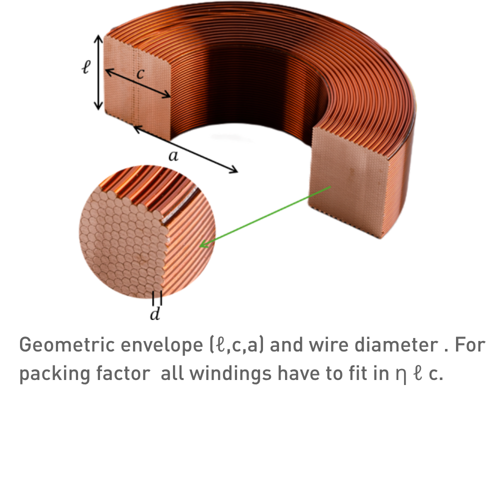
Every coil design starts with a set of geometric parameters that define the winding space. The winding space must contain all N turns. This gives the window constraint: $$ N \cdot A_w = \eta \cdot l \cdot c $$

$$ [\mathrm{m}^2] $$ This single equation links turns and wire diameter: for a given winding space (l,c) and packing factor (η), choosing N fixes d through wire cross section A_w and vice versa. For round wire $$ A_w = \frac{\pi d^2}{4} $$ Note that the mean bore radius a does not come in here. The critical consequence is that wire gauge cancels out of every figure of merit below. We will go over:

MMF and Motor/Lens Constants: what the coil does
Field Uniformity: how cleanly
Efficiency: for the least power and dissipation
Dynamical Aspects: how fast and the high-frequency wall

Wire gauge last

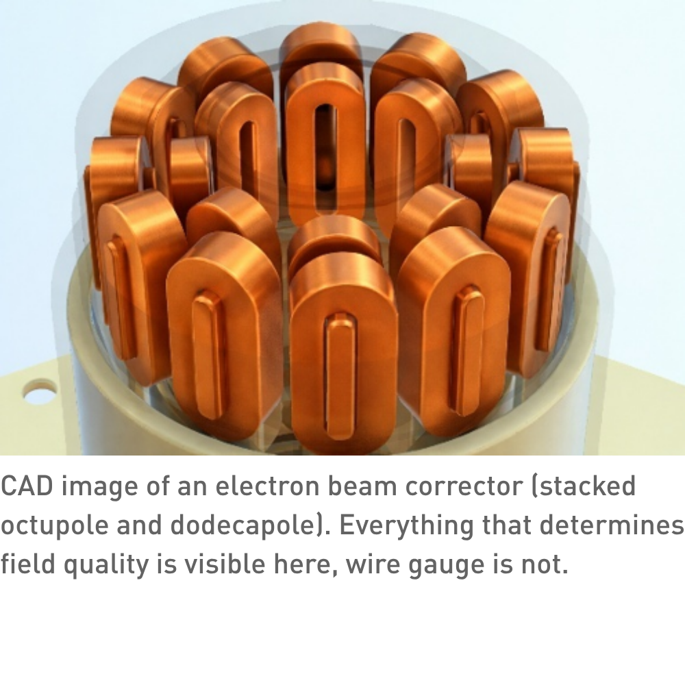
Every performance parameter — force, field, efficiency, bandwidth — depends on the winding geometry (a,c,ℓ), the packing factor (η), and the resistivity (ρ), but not on the particular combination of N and d used to fill the window. Wire gauge only determines the voltage-to-current ratio needed from the driver electronics. It is an impedance-matching decision, made after all performance parameters are fixed.

his is worth emphasising because many specifications lead with wire gauge and number of turns, as though these define the coil's capability. They do not. Two coils with identical geometry and packing factor but different N and d deliver identical MMF at identical power dissipation; they simply require different driver voltages. The functional specification should define what the coil must do (field, force, bandwidth, uniformity), not how the winding space is subdivided.

What the Coil Does: MMF and Motor/Lens Constants

Magnetomotive Force

$$ \mathrm{MMF} = N \cdot I \; [\mathrm{A} \cdot \text{turns}] $$ MMF is the source of all magnetic fields. For a given magnetic circuit geometry, NI determines B. Under constant NI, changing wire gauge only trades voltage for current without affecting field or force. MMF appears as the primary driver in all field-generating applications — magnets, beam optics, correctors, sensors, actuators — and should be the first item in any coil specification.

Motor and Lens Constants

The constant linking the electromagnetic input to the mechanical or optical output is geometry-fixed and gauge-independent. It converts a field or current into a force, deflection, or focusing effect.

Type	Constant	Units	Output	Application
Lorentz actuator	$$ K = B\,L_{wire} $$	$$ \mathrm{N/A} $$	F = K · I	Voice coil, linear motor
Reluctance actuator	$$ K_r = \frac{A_{gap}}{2\mu_0} $$	$$ \frac{N}{T^2} $$	$$ F = K_r B^2 $$	Solenoid valve, VR stepper
Solenoid lens	$$ K_{sol} = \int B_z^2 \, dz $$	$$ T^2 \cdot m $$	$$ \frac{1}{f} = \frac{K_{sol}}{(2Bp)^2} $$	Electron-optical lenses
Multipole (order n)	$$ k_n = \frac{G_n}{Bp} $$	$$ \frac{1}{m^n} $$	$$ \Delta x = -k_n L \frac{x^{n-1}}{(n-1)!} $$	Beam steering (n=1), focusing (n=2), aberration correction (n≥3)

The Lorentz force constant K is linear in current — doubling I doubles force. The reluctance force constant K_r produces force proportional to B² — doubling field quadruples force. This distinction has profound consequences for efficiency and control, treated in detail in the companion paper Lorentz vs. Reluctance Actuators. For beam-optics applications, the multipole gradient G_n scales as B₀/a^(n-1), where B₀ is the pole-tip field (limited by iron saturation at ~1.5–2 T) and a is bore radius. Tighter bores produce stronger multipoles for the same pole-tip field, increasingly steeply for higher orders. The beam's magnetic rigidity Bρ = p/q [T·m] converts the integrated field into a trajectory angle or focal length: it is fixed by the beam energy, not the magnet.

Field Uniformity

The spatial quality of the magnetic field over the working volume. Uniformity and efficiency are in tension: a compact coil maximises B²/P but sacrifices field flatness.

Metric	Definition	Relevant for
Homogeneity $$ \frac{\Delta B}{B} $$	Peak-to-peak variation over working volume [ppm]	MRI, NMR, precision magnets
Nagaoka coefficient $$ K_N $$	Fraction of infinite-solenoid field; $$ K_N \rightarrow 1 \text{ for } \ell \gg 2a $$	Any finite solenoid
Gradient linearity $$ \frac{\Delta G}{G} $$	Deviation of dB/dx from ideal over FOV	MRI gradients, beam optics
Multipole content	Unwanted harmonic amplitudes relative to main field [ppm]
Good-field radius	Radius within which spec is met; typically 0.7–0.8 × bore	Beam optics aperture design

Field uniformity is managed by end-correction windings, shimming, or accepting a good-field region smaller than the physical bore. The coil cross-section geometry (see Coil Cross-Section Geometry) and winding precision (see Coil Winding Basics) directly determine the achievable uniformity.

Efficiency: Steepness and Fabry Factor

All efficiency figures of merit share the same structure: output²/power, independent of operating point and wire gauge. For driver selection, inductance, resistance, and their time-constant is important

Type	Figure of merit	Units	Scaling law
Lorentz actuator	$$ K_N \rightarrow 1 \text{ for } \ell \gg 2a $$	$$ \mathrm{\frac{N^2}{W}} $$	2× force → 4× power
Reluctance actuator	$$ \frac{S_r}{P} = \frac{F}{R} = \frac{K_r}{R}\left(\frac{\mu_0 N}{g}\right)^2 $$	$$ \frac{N}{W} $$	2× force → 2× power
Resistive magnet	$$ \frac{B^2}{P} = \frac{\mu_0^2 \eta G^2}{\rho a} $$	$$ \frac{T^2}{W} $$	2× field→ 4× power
Inductance factor	$$ A_z = \frac{L}{N^2} = \frac{\mu_0 \pi a^2}{\ell W} $$	$$ H $$	Geometry only
Resistance factor	$$ A_R = \frac{R}{N^2} = \frac{\rho A_{wg}}{\eta \,\ell\, c} $$	$$ \Omega $$	Geometry + resistivity ρ
Time constant	$$ \tau = \frac{L}{R} = \frac{\mu_0 \,\eta\, c}{\rho\, W}\,\frac{A}{P_{avg}} $$	$$ s $$	Geometry + resistivity ρ

The Fabry factor G is a dimensionless geometric integral over the winding cross-section, depending only on the aspect ratios c/a and l/a. It plays the same role for field-generating coils that Steepness S plays for actuators, i.e. a geometry-only constant setting achievable field per unit √power. All three figures of merit improve with winding volume (larger c) and better packing (η), and are degraded only by resistivity (ρ). The reluctance actuator's F/P advantage over the Lorentz F²/P reflects the different force laws (B² vs B·I), not a difference in coil quality. These are the right numbers for comparing coil designs. Two coils for the same application should be compared on Steepness or Fabry factor, not on resistance or inductance in isolation — those depend on the arbitrary N/d split. The Wheeler correction factor $$ W = 1 + 0.9\left(\frac{a}{\ell}\right) + 0.32\left(\frac{c}{\ell}\right) + 0.84\left(\frac{c}{a}\right) $$ is, accurate to ~1 % for practical coil geometries. W = 1 for an infinite solenoid; W > 1 for all real coils.

Electrical Time Constant τ

The time constant τ=L/R is a quasi-static result, and is actual conservative at higher frequencies, because the AC resistance increases, see Dynamical Specification. Notable the axial length l cancels in first order (enters only through W(a,l,c)).

Application	Key driver	Want τ	Rationale
Scanning / deflection coil	Slew rate	Small	Current must slew quickly so want a small time constant. Note that for a voltage headroom $$ V_s > I \cdot R $$ the slew rate is limited by $$ \frac{V_s}{L} $$ rather than I/τ, at a cost of higher power during slew. Standard practice in galvo drivers and scanning magnets.
Corrector / orbit coil	Stability	Large	Drift and ripple requirements set minimum quality factor Q = 2πfτ, so τ must be large and a larger coil is accepted. AC effects are typically irrelevant. For resonant operation, higher τ gives sharper resonance.
Precision actuator	Steepness	Small, but large accepted	Force requirement sets minimum steepness S, so c and l are maximized, and τ is accepted as a consequence (sets requirement on driver). Bandwidth is typically low enough that AC effects are irrelevant.
Non-copper coil	Resistivity	Depends	Optimize resistivity ρ if other materials are considered.

Q&A

Why does wire gauge cancel out of every figure of merit?

The window constraint (Nd² = "constant" ) means that for a given winding space, choosing more turns of finer wire or fewer turns of heavier wire changes N and d in lockstep. Every FOM depends on products like N²d² or NI (which equals N·V/R, and R scales as N²), and these products resolve to geometry, packing, and resistivity — d drops out. Gauge only determines whether you need a high-voltage/low-current or low-voltage/high-current driver to reach the same NI.

What is the Fabry factor and why should I care about it?

The Fabry factor G is a dimensionless number (typically 0.1–0.2 for practical coils) that captures how efficiently a particular winding cross-section geometry converts electrical power into magnetic field. It depends only on the aspect ratios c/a and l/a. When comparing two coil designs for the same application, the one with the higher G produces more field per watt — regardless of wire gauge, number of turns, or operating current. It is the single most useful number for benchmarking resistive magnet designs.

How do I choose between optimising τ and optimising Steepness — they seem to conflict?

They do conflict, and the application determines the priority. Steepness improves with winding volume (more copper), but more copper also increases inductance and therefore τ. For fast-scanning coils and galvanometers, τ (bandwidth) dominates — you accept lower steepness to achieve speed. For precision positioning or high-force actuators operating at lower bandwidth, steepness dominates — you accept slower response to get more force per watt. The cross-application table in §4 shows where each application falls.

Our current spec lists wire gauge, resistance, and number of turns. What should it list instead?

A functional specification should define what the coil must do, not how the winding space is subdivided. Start with the required MMF (or force, or field, or deflection), then specify the geometric envelope (bore, radial build, axial length), the efficiency target (Steepness or Fabry factor), and any dynamic requirements (bandwidth, slew rate, or operating frequency). Add field uniformity requirements if applicable. Wire gauge, resistance, and number of turns are manufacturing outputs that follow from these functional requirements — they belong on the production drawing, not in the performance specification.

Can the driver compensate for a high τ, or is it a hard limit like self-resonant frequency (SRF)?

Partially. Higher drive voltage forces current to slew at V_s/L rather than the natural I/τ. This "voltage headroom" is standard in galvo drivers and scanning magnet supplies. But $$ f_{SRF} $$ is truly hard: above it, the coil is capacitive and more voltage produces less current, not more.

Discover our custom-designed coil assemblies

We partner with our customers to engineer and manufacture high-quality coils assemblies. Through close collaboration, we tailor each solution to meet exact application requirements—ensuring reliability, performance, and seamless integration into advanced systems.

More information

Contact our expert Stefan Slot

Get expert advice on custom coil assemblies tailored to your application.